


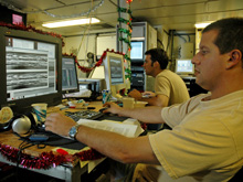
Sonar data systems specialist Akel Stirling and graduate student Jason Meyer process DSL120 sonar data in the shipboard computer lab. Click image for larger view and image credit.
Using Sound to "See" the Seafloor
December 20, 2005
Kelley Elliott
Web Coordinator
Akel Sterling
Senior Sonar Data Systems Specialist
Jennifer Morgan
Acoustic Data Specialist
Scott White
Assistant Professor and Co-PI
The DSL120 is back under tow, collecting data for days at a time. Data streaming in for scientific interpretation includes sonar data used to create sidescan imagery. Unlike air, water is not transparent, especially when it is thousands of meters deep. Light only travels about 100-300 feet in water, but sound can travel hundreds of miles under water. So to “see” the seafloor we make images using sound emitted from a sonar system. The raw data received on deck from the sonar, and the final resulting images, however, are two very different products. Acquiring and processing the data received from the sonar to produce a final image ready for geological interpretation is not simple, and we have a team of technicians from the Hawaii Mapping Research Group on board to conduct this process.
When a sound wave is emitted from a sidescan sonar, it spreads sideways and downwards from the system in an arc. When the sound wave strikes a solid surface, acoustic (sound) energy is scattered through the ocean, some of which is received back at the sonar. The DSL120 starts measuring time when each sonar wave is emitted, listening for the backscattered sounds. The strength of and time taken for each returned signal is recorded, and the data is sent through a live link to the surface for analysis. The data goes first through “bottom detect editing” where an acoustic specialist identifies the first returned sound, essentially removing the time taken for the sound to travel out and back through the water so the data reflects the seafloor terrain.
Next, corrections are applied to filter out “noise” or erroneous sound data. There is a lot of incidental sound in the ocean that may be picked up by the sonar, or an emitted sound wave might bounce off something other than the seafloor, such as a school of fish, showing up as unusual data. Usually the “noise” is obvious to the specialist looking at the data, but other times it may be hard to detect. Experience and knowledge helps us to differentiate between the good data and noise.
The strength of the received sound is normalized next by applying a “gain.” This is necessary because the farther the sound travels, both to and from the seafloor surface, the weaker the returned signal. So, for example, the sonar will receive a stronger returned signal from seafloor below it, while seafloor at the same depth but 30 meters to the side will return a weaker signal. This is much like the balance on your stereo. If you stand next to the left speaker you hear it stronger than the right, so to hear them equally you have to adjust the balance, reducing the left speaker and increasing the right speaker until they sound equal. So “angle varying gain” is applied to the data to balance out the returned sonar signal: the “gain” or volume is turned down on the data below the sonar head, and turned up farther away until they are balanced and all of the data can be evaluated equally.
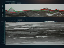
The screen grab above displays the first step in the sidescan sonar editing process, "bottom detect editing." The upper graph displays the magnitude per ping of returned sound recorded since the wave was emitted, by altitude as displayed on the Y axis, and ping along the X axis. During this phase of the process, an acoustic specialist identifies the first returned sound, essentially removing the time taken for the sound to travel out and back through the water so the data reflects the seafloor terrain. Click image for larger view and image credit.
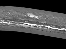
Once all variables are merged with the processed sound data, the complete dataset is georeferenced - converted from data with respect to time to data with respect to position. The final product is a grayscale image like the one seen above which can be used to make geological interpretations. In this image, the lighter colors display the weakest returned sounds, or shadows and less reflective surfaces, and the black are the strongest returns and harder surfaces. Click image for larger view and image credit.
After the data are adjusted based on the angle of the returned signal, gain is again applied based on the altitude of the sonar sled over the seafloor. A sonar receiver on the DSL120, flying 100- 125 meters off the bottom, times and receives all of the returned sound waves. So, a returned sound wave that travels through 100 meters of water will take less time and have a stronger returned signal when it is received than a sound wave that has to go through 125 meters of water. This is like the volume on your stereo. If you are 10 meters away from your stereo you can hear the volume louder than if you are 35 meters away, so to hear the sound as loud when you are 35 meters away you have to turn up the volume. The height of the sonar tow-sled above the seafloor is recorded continuously while it is underway, and this information is incorporated into the sonar data to normalize the values. “Gain” is applied to data collected when the DSL120 is higher off the bottom- the strength of the returned sound is ‘turned up’- so the strength of the signal displayed in the final image reflects the seafloor and not the altitude of the tow sled.
Last but not least, variations in the movement of the sonar tow-sled over the seafloor, namely navigation (geographical position), pitch, roll and heading, are merged with the processed sound data and the complete dataset is georeferenced - converted from data with respect to time to data with respect to position. Finally, a grayscale image is produced which can be used to make geological interpretations. The images are analogous to what would be seen if you shone a bright light across the seafloor if there were no water; the hard, shiny surfaces (like fresh lava) return the strongest signal and shadows return the weakest signal. On this cruise, the lighter colors display the weakest returned sounds, or shadows and less reflective surfaces, and the black are the strongest returns and more reflective surfaces. The final result are images that have converted all of the sound, time and variables into a black and white image that looks like a black and white photograph and can be used for scientific analysis.GalAPAGoS: Where Ridge Meets Hotspot will be sending reports from Dec 3 - Jan 10. Please check back frequently for additional logs from this expedition.
Sign up for the Ocean Explorer E-mail Update List.